Archive for the ‘finance’ Category

Variance swaps in a CAS

October 8, 2023

A couple of years ago I got a task of writing a module for pricing gamma swaps. I found the task quite difficult, as all I got to base on was an Excel spreadsheet with formulas that were clearly wrong and the few sources on the Internet that I found lacked details. This post (and maybe the next) describes things I learned at that time. Please keep in mind that I am not a quant – just a software guy, so it’s possible I got some of this wrong, maybe all. If you think this is the case please enlighten me in the comments.

One technique for solving problems is to find a practice problem – something easier, but similar enough that going through the exercise gives confidence that the method is sound and serves as a stepping stone to the more difficult one. In case of gamma swaps that simpler problem is pricing of variance swaps.

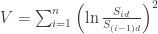
Variance swaps are financial instruments that are bets about the future observed variance of a price of an underlying asset. The parties that enter the contract observe the price S_t of the underlying at regular intervals d, i.e. at times

0=t_0<t_1=d<t_2=2d<...<t_n=nd=T,

where T is the life of the contract. Then they calculate the value V=\sum_{i=1}^n \left( \ln \frac{S_{id}}{S_{(i-1)d}}\right )^2 and settle the bet based on that value as compared to some predetermined “strike” value set in the contract. When pricing such contract the question is what is the fair value of the strike, i.e. what is the best prediction of it in the future based on what market tells us right now.

To answer this question suppose that the underlying price process is the geometric Brownian motion S_t = S_0\exp\left( \mu t + \sigma B_t\right), where \mu = \left(r - \frac{\sigma^2}{2} \right), r is the risk-free interest rate and B_t is the standard Brownian motion. Substituting that into the formula for V yields

V =  \sum_{i=1}^n \left(   \mu d + \sigma (B_{id}-B_{(i-1)d}) \right)^2

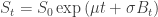
Taking the expectation on both sides we get

\mathbb{E} V = n(\mu d)^2 + \sigma^2 \sum_{i=1}^n \mathbb{E} (B_{id}-B_{(i-1)d})^2

(recall that \mathbb{E} (B_{id}-B_{(i-1)d}) = 0). Since B_{id}-B_{(i-1)d} has the same distribution as B_d and hence \mathbb{E} (B_{id}-B_{(i-1)d})^2 = \mathbb{E} (B_d)^2 for all i=1,...,n we get

\mathbb{E} V = n\left(r - \frac{\sigma^2}{2} \right)^2 d^2 + \sigma^2 T

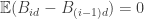
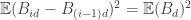
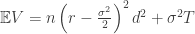
Now there is something I still don’t understand: in the pricing the first component is ignored – assumed equal to zero. Since typically d= 1/252year maybe indeed the value T \left(r - \frac{\sigma^2}{2} \right) ^2/252 is small enough to not matter.

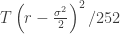
Anyway, whatever the rationale for ignoring that term is, as it was easy to guess the fair value of the variance swap strike is closely related to \sigma^2. The value of \sigma^2 can be obtained from option prices as implied volatility, but the problem is this way we actually get a different one for each strike. However, there is an interesting identity that provides a reasonable way to obtain a single number estimate for \sigma^2 from (interpolated) market option prices. Namely suppose that C(K) and P(K) are the prices of European call and put options with strike price K given by the Black-Scholes formula and F_0 = S_0 e^{rT}. Then the following identity holds:

(I) \int\limits_0^{F_0} \frac{1}{K^2}\ P(K) \, dK + \int\limits_{F_0}^\infty \frac{1}{K^2}\ C(K) \, dK  = \frac{T e^{-rT}}{2} \sigma^2

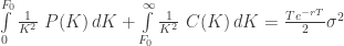
This way by interpolating (and extrapolating as needed) the actual market values of C(K) and P(K) we can get estimates of the integrals and after multiplying by \frac{2e^{rt}}{T} we know what we can expect V should be.

The rest of this post is about how to verify the identity above with Maxima Computer Algebra System (CAS).

(more…)