Variance swaps in a CAS

A couple of years ago I got a task of writing a module for pricing gamma swaps. I found the task quite difficult, as all I got to base on was an Excel spreadsheet with formulas that were clearly wrong and the few sources on the Internet that I found lacked details. This post (and maybe the next) describes things I learned at that time. Please keep in mind that I am not a quant – just a software guy, so it’s possible I got some of this wrong, maybe all. If you think this is the case please enlighten me in the comments.

One technique for solving problems is to find a practice problem – something easier, but similar enough that going through the exercise gives confidence that the method is sound and serves as a stepping stone to the more difficult one. In case of gamma swaps that simpler problem is pricing of variance swaps.

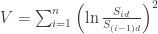
Variance swaps are financial instruments that are bets about the future observed variance of a price of an underlying asset. The parties that enter the contract observe the price $S_t$ of the underlying at regular intervals $d$ , i.e. at times

$0=t_0<t_1=d<t_2=2d<...<t_n=nd=T$ ,

where $T$ is the life of the contract. Then they calculate the value $V=\sum_{i=1}^n \left( \ln \frac{S_{id}}{S_{(i-1)d}}\right )^2$ and settle the bet based on that value as compared to some predetermined “strike” value set in the contract. When pricing such contract the question is what is the fair value of the strike, i.e. what is the best prediction of it in the future based on what market tells us right now.

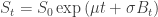
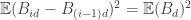
To answer this question suppose that the underlying price process is the geometric Brownian motion $S_t = S_0\exp\left( \mu t + \sigma B_t\right)$ , where $\mu = \left(r - \frac{\sigma^2}{2} \right)$ , $r$ is the risk-free interest rate and $B_t$ is the standard Brownian motion. Substituting that into the formula for $V$ yields

$V = \sum_{i=1}^n \left( \mu d + \sigma (B_{id}-B_{(i-1)d}) \right)^2$

Taking the expectation on both sides we get

$\mathbb{E} V = n(\mu d)^2 + \sigma^2 \sum_{i=1}^n \mathbb{E} (B_{id}-B_{(i-1)d})^2$

(recall that 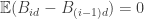$\mathbb{E} (B_{id}-B_{(i-1)d}) = 0$ ). Since $B_{id}-B_{(i-1)d}$ has the same distribution as $B_d$ and hence $\mathbb{E} (B_{id}-B_{(i-1)d})^2 = \mathbb{E} (B_d)^2$ for all $i=1,...,n$ we get

$\mathbb{E} V = n\left(r - \frac{\sigma^2}{2} \right)^2 d^2 + \sigma^2 T$

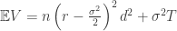
Now there is something I still don’t understand: in the pricing the first component is ignored – assumed equal to zero. Since typically $d= 1/252$ year maybe indeed the value $T \left(r - \frac{\sigma^2}{2} \right) ^2/252$ is small enough to not matter.

Anyway, whatever the rationale for ignoring that term is, as it was easy to guess the fair value of the variance swap strike is closely related to $\sigma^2$ . The value of $\sigma^2$ can be obtained from option prices as implied volatility, but the problem is this way we actually get a different one for each strike. However, there is an interesting identity that provides a reasonable way to obtain a single number estimate for $\sigma^2$ from (interpolated) market option prices. Namely suppose that $C(K)$ and $P(K)$ are the prices of European call and put options with strike price $K$ given by the Black-Scholes formula and $F_0 = S_0 e^{rT}$ . Then the following identity holds:

(I) $\int\limits_0^{F_0} \frac{1}{K^2}\ P(K) \, dK + \int\limits_{F_0}^\infty \frac{1}{K^2}\ C(K) \, dK = \frac{T e^{-rT}}{2} \sigma^2$

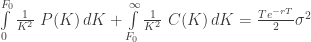
This way by interpolating (and extrapolating as needed) the actual market values of $C(K)$ and $P(K)$ we can get estimates of the integrals and after multiplying by $\frac{2e^{rt}}{T}$ we know what we can expect $V$ should be.

The rest of this post is about how to verify the identity above with Maxima Computer Algebra System (CAS).

The first step is to define the Black-Scholes formulas for prices of Eropean call and put options:

assume(T>0,S>0,σ>0,r>0);
CN(x) := (1+erf(x/sqrt(2)))/2;
d1 : (log(S/K) + (r+σ^2/2)*T)/(σ*sqrt(T));
d2 : d1-σ*sqrt(T);
C : ratsimp(CN(d1)*S-CN(d2)*K*exp(-r*T));
P: ratsimp(CN(-d2)*K*exp(-r*T) - CN(-d1)*S);

Maxima can compute definite integrals, so it would be nice to just tell it to calculate the integrals in the (I) identity and be done. This fails however, apparently the task is beyond what Maxima can do. However, it is able to calculate the antiderivatives of $K\mapsto C(K)/K^2$ and $K\mapsto P(K)/K^2$ , so this is how we work around the limitation. First we calculate the antiderivative related to the call price:

logexpand:super;
CiK2:expand(integrate(C/K^2, K))

The result is too long to quote here in whole, but it is a sum of nine components:

C1:part(CiK2,1);
C2:part(CiK2,2);
C3:part(CiK2,3);
C4:part(CiK2,4);
C5:part(CiK2,5);
C6:part(CiK2,6);
C7:part(CiK2,7);
C8:part(CiK2,8);
C9:part(CiK2,9);

Those components are as follows (Maxima can export to LaTex, I just needed to replace \operatorname with \text ):

1: $-\frac{S \text{erf}\left( \frac{\sqrt{T} \sigma }{{{2}^{\frac{3}{2}}}}+\frac{\sqrt{T} r}{\sqrt{2} \sigma }+\frac{\log{(S)}}{\sqrt{2} \sqrt{T} \sigma }-\frac{\log{(K)}}{\sqrt{2} \sqrt{T} \sigma }\right) }{2 K}$

2: $-\frac{{{S}^{\frac{1}{2}-\frac{r}{{{\sigma }^{2}}}}} {{e}^{\frac{\log{(S)} r}{{{\sigma }^{2}}}-T r-\frac{\log{(S)}}{2}}} \text{erf}\left( \frac{\sqrt{T} \sigma }{{{2}^{\frac{3}{2}}}}-\frac{\sqrt{T} r}{\sqrt{2} \sigma }-\frac{\log{(S)}}{\sqrt{2} \sqrt{T} \sigma }+\frac{\log{(K)}}{\sqrt{2} \sqrt{T} \sigma }\right) }{2}$

3: $\frac{T {{e}^{-T r}} {{\sigma }^{2}} \text{erf}\left( \frac{\sqrt{T} \sigma }{{{2}^{\frac{3}{2}}}}-\frac{\sqrt{T} r}{\sqrt{2} \sigma }-\frac{\log{(S)}}{\sqrt{2} \sqrt{T} \sigma }+\frac{\log{(K)}}{\sqrt{2} \sqrt{T} \sigma }\right) }{4}$

4: $-\frac{T r {{e}^{-T r}} \text{erf}\left( \frac{\sqrt{T} \sigma }{{{2}^{\frac{3}{2}}}}-\frac{\sqrt{T} r}{\sqrt{2} \sigma }-\frac{\log{(S)}}{\sqrt{2} \sqrt{T} \sigma }+\frac{\log{(K)}}{\sqrt{2} \sqrt{T} \sigma }\right) }{2}$

5: $-\frac{\log{(S)} {{e}^{-T r}} \text{erf}\left( \frac{\sqrt{T} \sigma }{{{2}^{\frac{3}{2}}}}-\frac{\sqrt{T} r}{\sqrt{2} \sigma }-\frac{\log{(S)}}{\sqrt{2} \sqrt{T} \sigma }+\frac{\log{(K)}}{\sqrt{2} \sqrt{T} \sigma }\right) }{2}$

6: $\frac{\log{(K)} {{e}^{-T r}} \text{erf}\left( \frac{\sqrt{T} \sigma }{{{2}^{\frac{3}{2}}}}-\frac{\sqrt{T} r}{\sqrt{2} \sigma }-\frac{\log{(S)}}{\sqrt{2} \sqrt{T} \sigma }+\frac{\log{(K)}}{\sqrt{2} \sqrt{T} \sigma }\right) }{2}$

7: $\frac{\sqrt{T} \sigma {{e}^{-\frac{T {{\sigma }^{2}}}{8}-\frac{T {{r}^{2}}}{2 {{\sigma }^{2}}}-\frac{\log{(S)} r}{{{\sigma }^{2}}}+\frac{\log{(K)} r}{{{\sigma }^{2}}}-\frac{{{\log{(S)}}^{2}}}{2 T {{\sigma }^{2}}}+\frac{\log{(K)} \log{(S)}}{T {{\sigma }^{2}}}-\frac{{{\log{(K)}}^{2}}}{2 T {{\sigma }^{2}}}-\frac{T r}{2}+\frac{\log{(S)}}{2}-\frac{\log{(K)}}{2}}}}{\sqrt{2} \sqrt{\pi }}$

8: $-\frac{\log{(K)} {{e}^{-T r}}}{2}$

9: $-\frac{S}{2 K}$

Just in case, let’s check if Maxima is sure the sum of these expressions is the same as the original integral:

is(equal(CiK2,C1+C2+C3+C4+C5+C6+C7+C8+C9));

Maxima responds “true”, so it must be. The formulas do not look tractable, but fear not. Let’s see how these terms behave as $K \rightarrow \infty$ :

C1L:limit(C1, K, inf);
C2L:limit(C2, K, inf);
C3L:limit(C3, K, inf);
C4L:limit(C4, K, inf);
C5L:limit(C5, K, inf);
C6L:limit(C6, K, inf);
C7L:limit(C7, K, inf);
C8L:limit(C8, K, inf);
C9L:limit(C9, K, inf);

These nine limits turn out to be

1: 0

2: $-\frac{{{S}^{\frac{1}{2}-\frac{r}{{{\sigma }^{2}}}}} {{\% e}^{\frac{\log{(S)} r}{{{\sigma }^{2}}}-T r-\frac{\log{(S)}}{2}}}}{2}$

3: $\frac{T {{e}^{-T r}} {{\sigma }^{2}}}{4}$

4: $-\frac{T r {{e}^{-T r}}}{2}$

5: $-\frac{\log{(S)} {{e}^{-T r}}}{2}$

6: $\infty$

7: 0

8: $-\infty$

9: 0

That does not look so bad, except for the limits 6 and 8 that are not finite. Fortunately the limit of the sum of the corresponding components is 0, so they cancel out at infinity:

C68L:limit(C6+C8, K, inf);
0

The second limit can be simplified:

radcan(C2L);

$-\frac{{{e}^{-T r}}}{2}$

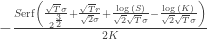
So, we can compute the limit of the whole expression as

CIK2L:factor(C1L+radcan(C2L)+C3L+C4L+C5L+C68L+C7L+C9L);

Which gives:

$\frac{{{e}^{-T r}} \left( T {{\sigma }^{2}}-2 T r-2 \log{(S)}-2\right) }{4}$

To get the integral from $F=S e^{rT}$ to infinity we need the value of CiK2 at $F$ .

F:S*exp(T*r);
CIK2F:subst(K=F,CiK2);

After adding some simplification code

CIK2Fs:expand(radcan(CIK2F));
factor_out(e1,e2):=if not is(op(e2)="+")  then e2 else e1*apply("+",map(lambda([x],x/e1), args(e2)));
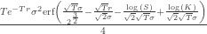
CIK2Fsf:factor_out(%e^(-T*r),CIK2Fs);

we get formula for CIK2Fsf to be

${{e}^{-T r}} \left( \frac{T {{\sigma }^{2}} \text{erf}\left( \frac{\sqrt{T} \sigma }{{{2}^{\frac{3}{2}}}}\right) }{4}-\text{erf}\left( \frac{\sqrt{T} \sigma }{{{2}^{\frac{3}{2}}}}\right) +\frac{\sqrt{T} \sigma {{\% e}^{-\frac{T {{\sigma }^{2}}}{8}}}}{\sqrt{2} \sqrt{\pi }}-\frac{T r}{2}-\frac{\log{(S)}}{2}-\frac{1}{2}\right)$

To check if the simplification code was ok we can do

is(equal(CIK2Fsf,CIK2Fs))
true

Now we can compute the integral from $F=S e^{rT}$ to infinity:

CI:factor_out(%e^(-T*r),CIK2L-CIK2Fsf)
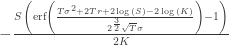
CIs:substpart(expand(part(CI,2)),CI,2);

and we obtain the call option integral of the identity as

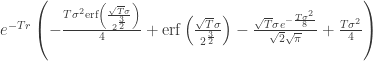
${{e}^{-T r}} \left( -\frac{T {{\sigma }^{2}} \text{erf}\left( \frac{\sqrt{T} \sigma }{{{2}^{\frac{3}{2}}}}\right) }{4}+\text{erf}\left( \frac{\sqrt{T} \sigma }{{{2}^{\frac{3}{2}}}}\right) -\frac{\sqrt{T} \sigma {{e}^{-\frac{T {{\sigma }^{2}}}{8}}}}{\sqrt{2} \sqrt{\pi }}+\frac{T {{\sigma }^{2}}}{4}\right)$

Not nice, but not that horrible either.

Now it’s time to do the integral $\int\limits_0^{F_0} \frac{1}{K^2}\ P(K) \, dK$ . Again Maxima fails to evaluate this directly, but is able to compute the antiderivative that is a sum of nine components:

PiK2:expand(integrate(P/K^2, K));
P1:part(PiK2,1);
P2:part(PiK2,2);
P3:part(PiK2,3);
P4:part(PiK2,4);
P5:part(PiK2,5);
P6:part(PiK2,6);
P7:part(PiK2,7);
P8:part(PiK2,8);
P9:part(PiK2,9);

Let’s check if we have all the components of the sum:

is(equal(PiK2,P1+P2+P3+P4+P5+P6+P7+P8+P9));
true

Now let’s compute the limits of the components at 0.

P1L:limit(P1, K, 0,plus);
P2L:limit(P2, K, 0,plus);
P3L:limit(P3, K, 0,plus);
P4L:limit(P4, K, 0,plus);
P5L:limit(P5, K, 0,plus);
P6L:limit(P6, K, 0,plus);
P7L:limit(P7, K, 0,plus);
P8L:limit(P8, K, 0,plus);
P9L:limit(P9, K, 0,plus);

This gives us the following limits:

1: $-\infty$

2: $\frac{{{S}^{\frac{1}{2}-\frac{r}{{{\sigma }^{2}}}}} {{e}^{\frac{\log{(S)} r}{{{\sigma }^{2}}}-T r-\frac{\log{(S)}}{2}}}}{2}$

3: $-\frac{T {{e}^{-T r}} {{\sigma }^{2}}}{4}$

4: $\frac{T r {{\% e}^{-T r}}}{2}$

5: $\frac{\log{(S)} {{\% e}^{-T r}}}{2}$

6: $\infty$

7: 0

8: $-\infty$

9: $\infty$

Again we try to group the problematic limits so that we get finite values. First, we can show that limit of P6+P8 at 0 is 0:

P68L:limit(factor(P6+P8),K,0,plus);
0

The limit of P1+P9 is a bit more difficult.

fP1P9:factor(P1+P9);

This gives us that P1+P9 is

$-\frac{S\, \left( \text{erf}\left( \frac{T {{\sigma }^{2}}+2 T r+2 \log{(S)}-2 \log{(K)}}{{{2}^{\frac{3}{2}}} \sqrt{T} \sigma }\right) -1\right) }{2 K}$ .

Now denote the $\text{erf}\left( \frac{T {{\sigma }^{2}}+2 T r+2 \log{(S)}-2 \log{(K)}}{{{2}^{\frac{3}{2}}} \sqrt{T} \sigma }\right)$ part of this expression as $X$ so that P1+P9 can be written as $-S \frac{X-1}{2 K}$ :

X:part(fP1P9,1,1,2,1);
is(equal(factor(P1+P9),-S*(X-1)/(2*K)));
true

Turns out, the right limit of X at 0 is 1:

limit(X, K, 0, plus);
1

Hence we can apply L’Hôpital’s rule to calculate the limit of P1+P9 at 0:

P19L:-S*limit(diff(X-1,K),K,0,plus)/2;

which turns out to be 0.

Finally we have the following for the limit of the put integral at 0:

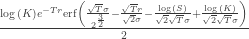
PIK2L:factor_out(%e^(-T*r),P19L+P2L+P3L+P4L+P5L+P68L+P7L);

which gives

${{e}^{-T r}} \left( \frac{{{S}^{\frac{1}{2}-\frac{r}{{{\sigma }^{2}}}}} {{e}^{\frac{\log{(S)} r}{{{\sigma }^{2}}}-\frac{\log{(S)}}{2}}}}{2}-\frac{T {{\sigma }^{2}}}{4}+\frac{T r}{2}+\frac{\log{(S)}}{2}\right)$

The antiderivative PiK2 of $K\mapsto P(K)/K^2$ at the forward price $F=S e^{r T}$ is

PIK2F:subst(K=F,PiK2);
PIK2Fs:expand(radcan(PIK2F));

$\frac{T {{e}^{-T r}} {{\sigma }^{2}} \text{erf}\left( \frac{\sqrt{T} \sigma }{{{2}^{\frac{3}{2}}}}\right) }{4}-{{e}^{-T r}} \text{erf}\left( \frac{\sqrt{T} \sigma }{{{2}^{\frac{3}{2}}}}\right) +\frac{\sqrt{T} \sigma {{e}^{-\frac{T {{\sigma }^{2}}}{8}-T r}}}{\sqrt{2} \sqrt{\pi }}+\frac{T r {{e}^{-T r}}}{2}+\frac{\log{(S)} {{e}^{-T r}}}{2}+\frac{{{e}^{-T r}}}{2}$

So the definite integral corresponding to put options in the identity (I) is

PI:factor_out(%e^(-T*r),PIK2Fs-PIK2L);

${{e}^{-T r}} \left( \frac{T {{\sigma }^{2}} \text{erf}\left( \frac{\sqrt{T} \sigma }{{{2}^{\frac{3}{2}}}}\right) }{4}-\text{erf}\left( \frac{\sqrt{T} \sigma }{{{2}^{\frac{3}{2}}}}\right) +\frac{\sqrt{T} \sigma {{e}^{-\frac{T {{\sigma }^{2}}}{8}}}}{\sqrt{2} \sqrt{\pi }}-\frac{{{S}^{\frac{1}{2}-\frac{r}{{{\sigma }^{2}}}}} {{e}^{\frac{\log{(S)} r}{{{\sigma }^{2}}}-\frac{\log{(S)}}{2}}}}{2}+\frac{T {{\sigma }^{2}}}{4}+\frac{1}{2}\right)$

We add that to the formula for the call part obtained above and the miracle happens:

VS:radcan(PI+CI);

$\frac{T {{e}^{-T r}} {{\sigma }^{2}}}{2}$

QED

Tags: Maxima, Variance swaps

This entry was posted on October 8, 2023 at 5:01 pm and is filed under finance. You can follow any responses to this entry through the RSS 2.0 feed. You can leave a response, or trackback from your own site.

Formalized Mathematics